The first article ignored the effect of air friction on the pumpkin's flight. This enabled us to gain a rough idea of the kind of speeds that are involved in throwing a pumpkin 4000 feet (1219m) or more.

The second article showed that air friction was significant, and we developed equations that describe the effect of this friction.

Now, we want to look at what these equations predict. We have two questions still unanswered: How fast does a pumpkin have to be thrown to reach 4000 feet? And what is the best angle of elevation?

When we ignored air resistance, we predicted that we needed a muzzle velocity of 393 km/hour when using the optimum angle of elevation of 45 degrees. Let's plot this first.

UltimaCalc contains a very flexible, general-purpose tool for creating plots of functions. A plot is based on a 4 step process:

• Specify initial conditions.
• Specify a termination condition.
• Specify the calculation(s) to be performed at each iteration. In particular, calculate the values of the variables x and y.
• Specify how variables change after each iteration.

Here is a screen shot of this tool:

UltimaCalc draws a plot by first performing the set of instructions that specify the initial conditions. In our example, we need to specify the muzzle velocity V₀ (calculated as 109.34 m/s in the first article, about 394 km/hour) and the angle of elevation a. We also need to initialise x and y to 0. The plot will be drawn at small time increments. Let's set the time, t, to 0 and the time interval that each iteration represents, or dt, to a suitable value. As yet, we don't know what might be a suitable value, so let's choose 1 second. It's also convenient to specify the acceleration due to gravity here.

We enter all this as a set of expressions, separated by either commas or semicolons:

V0 = 109.34; a = 45; x = 0; y = 0; t = 0; dt = 1; g = 9.80665;

We also need to set the initial values of the two components of the velocity. (The asterisk represents a multiplication sign.) Notice that we don't put a semicolon after the final item:

Vx = V0*cos(a); Vy = V0*sin(a)

We don't know how long the pumpkin will be in the air, but we do know that its flight ends when it hits the ground. It is therefore in the air while y is greater than or equal to 0:

y >= 0

The pumpkin moves horizontally at a constant velocity. At each iteration, its distance from the muzzle increases by V_x.dt. Its vertical velocity V_y changes due to the force of gravity, decreasing by g.dt per iteration.

Its height increases by approximately (V_y - g.dt/2).dt, being its average vertical speed over the interval multiplied by the time duration of the interval. The value of V_y used here when calculating y is its value before it is iterated. Thus we have:

x = x + Vx*dt; y = y + (V_y - g*dt/2)*dt; Vy = Vy - g*dt

This is easy. All we need to do is to advance the time:

t = t + dt

OK, let's see what happens. First, click on the 'Show x, y' check box to include the initial values of x and y in the plot. Also click on the 'Deg' check box to indicate that we are calculating with angles in degrees. (Both checkboxes should now have ticks in them.) Click on the Plot button (or hit the Enter key).

The result looks pretty good, except that it is clearly made up of a series of straight lines, especially noticeable at the top of the curve. However, the estimated range seems to be close to our target of 1219m. If we halve the time interval, changing dt to 0.5, the curve looks smoother, but the range has changed very slightly. Making dt even smaller seems to have little effect.

We can verify that we have the optimum angle of elevation. Changing the value of a to 40 causes a reduction in the range. So does changing it to 50. The little crosses on the plot indicate the points which were calculated. They are evenly spaced in the horizontal direction.

So far so good. But we already know that assuming zero air resistance is not a reasonable choice.

In the previous article, we estimated the amount of drag due to air resistance and found expressions for the vertical and horizontal accelerations caused by this. Let's create a new plot, so we can compare the old with the new very easily.

First, copy all of the entries we made to Plot 1. Copy the initial conditions, click on the 'Plot 2' tab, and paste them as the initial conditions for the new plot. Do the same for the three other texts. Click in the two checkboxes so that they both show ticks.

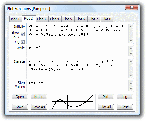
Now we modify the second plot. To the initial conditions, we need to add an entry, the value of k. This is the ratio of drag to the square of the speed, and was calculated as:

k = 1/2 * density of medium * reference area * drag coefficient.

Using our previous estimates for the reference area and drag coefficient, we can calculate this to be about 0.0013. Add this to the list of initial conditions by adding a semicolon followed by k = 0.0013.

We also modify the list of iteration expressions. Remove the term Vy = Vy - g*dt and replace it with:

Vx = Vx - k*Vx*vx; Vy = Vy - k*Vy*abs(Vy)*dt - g*dt

Now click on the 'Plot' button or hit the 'Enter' key.

The obvious change is that the plot is no longer symmetrical. The point of maximum height is no longer half way along. Look at the markings on the axes. The range is nothing like 1200m - it is only 658m. The maximum height reached is only 223m, compared with 305m previously.

The small crosses showing the calculated points are now closer together on the right, indicating that the pumpkin is travelling a shorter and shorter distance in each interval. If you like, you can turn off these markers. Do a right click on the plot and select 'Set Display Properties' in the menu that pops up. A 'Plot Options' window appears. Click on the 'Markers' tab, click on 'None', and click 'OK'.

We need to test whether we are calculating at short enough time intervals. Try reducing the value of dt to 0.1. The estimated range increases slightly to 659m, so try a value of 0.05sec. The range increases again, but not by much.

For a really striking comparison, click on the 'Plot All' button to see the two plots together. The difference is dramatic.

Clearly, to reach 1200m or so, we need a much greater initial velocity. Increase V0 until the two plots end at the same point. With a muzzle velocity of 206m/s, the range is 1220m.

Observing the two plots together, the second one now travels higher, suggesting that perhaps a lower angle of elevation might be beneficial. Let's play with the angle of elevation, a, which we set at 45 degrees, the optimum when air friction is not significant. The range increases if the elevation is reduced slightly, the best being 1236m at an elevation of around 38 degrees. At this elevation, a muzzle velocity of 203m/s is enough to achieve our target range.

If we take the simple approach, we can quite easily calculate that we can through a pumpkin a distance of 4000 feet (1219 metres) by shooting it at a velocity of 109.34m/s (245mph) at precisely 45 degrees to the horizontal. The pumpkin in this situation would follow a parabolic path.

With air resistance slowing it down, the pumpkin actually needs a greater muzzle velocity, estimated as 203m/s (454mph). The trajectory is no longer parabolic, and the optimum angle of elevation is slightly lower, at around 38 degrees.

These figures seem to be quite realistic. However, I made a number of crude estimates in the previous article, If someone can give more accurate figures for the pumpkin's dimensions, weight, muzzle velocity and range, we would be glad to hear from you.

What happens if we can make the muzzle velocity much greater (without the pumpkin being destroyed, which would be a failed attempt)?

A muzzle velocity of 500m/s and elevation of 32 degrees give a range of 2125m. Notice the peculiarity of the trajectory initially curving upwards, rather than downwards. This seems to be due to a greater drag in the horizontal direction, due to the horizontal speed being greater that the vertical speed by about 40%, and the horizontal component of the drag being about double the vertical component of the drag.

The estimated terminal velocity, from the previous article, is about 107m/s. This is the speed at which the vertical drag equals its weight. Here, the inital vertical velocity is 265m/s. The drag as it climbs is six times its weight! The horizontal drag is approaching 16 times its weight. The calculation markers confirm this rapid deceleration. Even if the pumpkin could be safely accelerated to this speed, I question whether it would stand up to the force of the drag acting on it as soon as it leaves the cannon.

The asymmetry is very marked, the pumpkin falling very steeply at the end of its flight. In the old days, it was believed that a cannon ball would fly until it was over its target, then drop suddenly on to it. When I first read about this belief, the author ridiculed it. But here, we have the same kind of thing happening.

We could try higher and higher speeds. However, the pumpkin in our last experiment was already exceeding the speed of sound, casting doubt as to whether the math applies in this case. Perhaps it is time to move on...